Phase 1: Understanding Aerodynamic Forces and Coefficients

Aerodynamics is the study of how air interacts with moving objects. For aircraft, the introductory results are lift, drag, aerodynamic moments, and pressure changes around wings and bodies. An aerodynamics calculator organizes these relationships by combining air density, speed, reference area, geometry, and aerodynamic coefficients. The calculator does not create the physics; it applies a mathematical model to the supplied inputs. That distinction matters because one aircraft can produce very different forces at different speeds, angles of attack, altitudes, and configurations. A useful calculation therefore begins by defining the flight condition, selecting consistent units, and understanding what each coefficient represents.

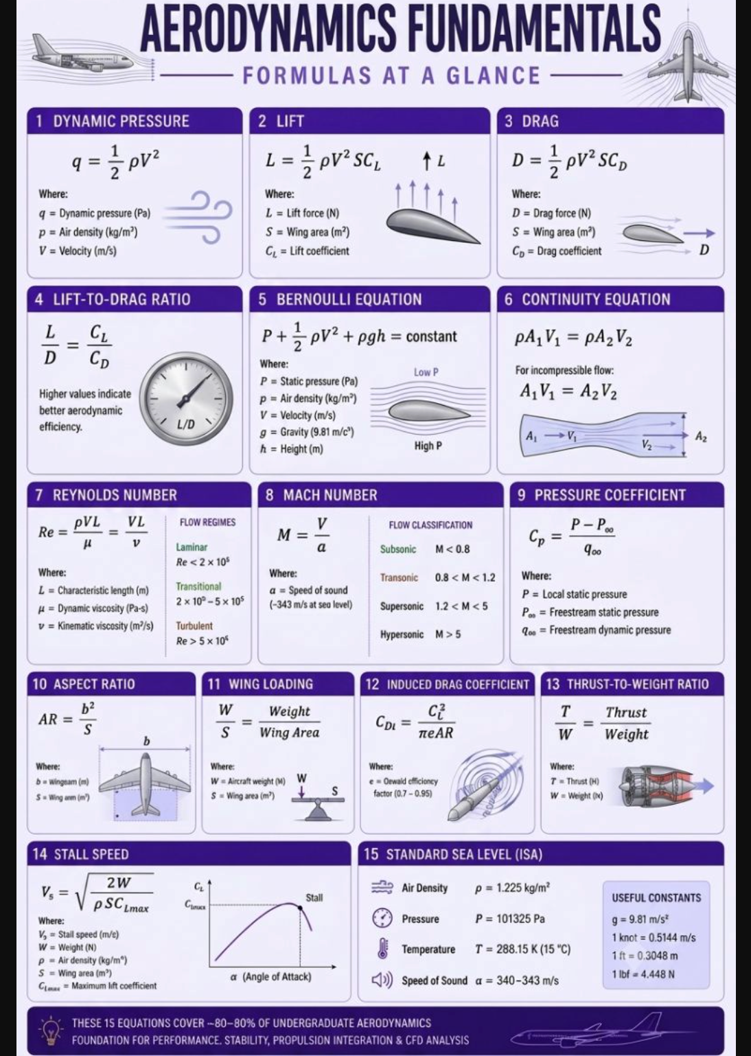
The standard lift equation is L = 0.5 × ρ × V² × S × C_L. Here, L is lift, ρ is air density, V is speed relative to the surrounding air, S is wing reference area, and C_L is the lift coefficient. The factor 0.5 × ρ × V² is dynamic pressure and is commonly written q, so the equation becomes L = qSC_L. NASA explains that the lift coefficient collects complicated effects involving shape, inclination, viscosity, and compressibility into one value. That convenience does not make C_L a universal constant; it must match the aerodynamic condition being analyzed. It remains meaningful only when those underlying conditions are compatible.

Drag uses the related equation D = 0.5 × ρ × V² × S × C_D, or D = qSC_D. The symbols have the same meanings, except C_D is the drag coefficient. Drag acts opposite the relative airflow and represents resistance to motion through the air. NASA notes that drag depends on density, velocity, viscosity, compressibility, size, shape, and orientation. The reference area used with C_D must match the convention used when the coefficient was determined. Aircraft data often use wing planform area, but other objects may use frontal or wetted area, making source checking essential. Otherwise, the resulting drag calculation may look precise while using mismatched definitions.

Dynamic pressure deserves special attention because it appears throughout aerodynamic analysis. The equation q = 0.5 × ρ × V² shows that dynamic pressure depends linearly on density and on the square of velocity. If density remains constant and speed doubles, dynamic pressure becomes four times as large. If coefficient and reference area also remain unchanged, calculated lift or drag becomes four times as large. Real aircraft may not keep their coefficients constant as speed changes because angle of attack, Reynolds number, Mach number, or configuration may also change. Even so, dynamic pressure explains why aerodynamic loads often rise rapidly with airspeed significantly.

Consider a simple lift example. Suppose an aircraft flies where air density is 0.0020 slug per cubic foot, true airspeed is 150 feet per second, wing area is 180 square feet, and C_L is 0.60. First calculate dynamic pressure: q = 0.5 × 0.0020 × 150². Because 150² is 22,500, q equals 22.5 pounds per square foot. Lift is 22.5 × 180 × 0.60, which equals 2,430 pounds-force. Under these assumptions, the wing produces about 2,430 pounds of lift. If aircraft weight is also about 2,430 pounds, the result is consistent with steady level flight at that instant in the model.

The same condition can estimate drag if a compatible drag coefficient is known. Assume C_D = 0.040 and retain the 22.5 pounds-per-square-foot dynamic pressure and 180-square-foot reference area. Drag becomes 22.5 × 180 × 0.040, or 162 pounds-force. The lift-to-drag ratio is therefore 2,430 ÷ 162 = 15. Because q and S appear in both equations, the ratio can also be calculated as C_L/C_D, giving 0.60 ÷ 0.040 = 15. Higher L/D generally indicates greater aerodynamic efficiency, although maximum L/D is not automatically the best condition for maximum speed, minimum time, or every mission objective considered.

Angle of attack is the angle between an airfoil’s reference chord line and the relative airflow. For many airfoils in ordinary attached-flow conditions, increasing angle of attack increases lift coefficient approximately linearly through part of the operating range. That trend does not continue indefinitely. Near a critical angle, airflow can separate strongly from the surface and the airfoil can stall, causing lift coefficient to stop increasing and then decrease. The critical angle depends on airfoil shape, Reynolds number, Mach number, contamination, and configuration. An airfoil analysis tool therefore needs more information than angle of attack alone for reliable wide-range predictions.

Aerodynamic coefficients let engineers compare shapes and test results without relying only on raw force measurements. Lift coefficient can be calculated from C_L = L/(qS), while drag coefficient follows C_D = D/(qS). These coefficients are dimensionless, but their values still depend on test conditions and chosen reference quantities. NASA emphasizes that coefficient transfer requires similar flow conditions. Reynolds number describes the balance between inertial and viscous effects, while Mach number compares flow speed with the speed of sound. Large differences in either parameter can make data measured in one experiment unsuitable for another case, even when the geometry appears unchanged.

Reference geometry must also remain consistent. Wing area usually means planform area rather than the total physical surface of the upper and lower skins. Chord is a characteristic front-to-back dimension, while span measures wingtip-to-wingtip distance. Aspect ratio relates span and area and influences induced drag. Aerodynamic moments require both a reference chord and a reference point. These definitions may appear administrative, yet they determine the numerical meaning of each coefficient. Two reports can give different coefficients for the same force because they use different areas, lengths, or moment references. A calculator should therefore state conventions instead of assuming universal definitions.

Calculation Portal’s aerodynamics tools are best used as transparent analysis aids. Start with the quantity needed, identify the governing equation, and confirm that density, velocity, area, and coefficients describe the same condition. Then use the calculator to validate units, repeat calculations, and compare scenarios. The related atmosphere section provides environmental properties, while aircraft performance, flight mechanics, and stability show how aerodynamic forces affect the complete aircraft. Results should be treated as estimates whenever simplified coefficients or idealized flow assumptions are used. For certified operations, structural limits, or professional design decisions, rely on validated data and approved documentation for the specific aircraft or vehicle.

Phase 2: Airfoils, Lift, Drag, and Pressure Distribution

Lift and drag are not produced by one cause; they emerge from the pressure and shear stresses acting over an aircraft’s surface. Air moving around a wing changes speed and direction, creating a pressure distribution that differs between the upper and lower surfaces. Viscosity also produces tangential shear at the surface. When these local effects are integrated over the entire wing, the resulting force can be resolved into lift and drag. This viewpoint is more complete than saying a wing creates lift only because air moves faster over one side. Real aerodynamic force reflects conservation of momentum, pressure variation, circulation, viscosity, and three-dimensional flow together.

An airfoil is a section shape used to study wing behavior. Its leading edge faces the oncoming flow, its trailing edge lies at the rear, and the chord line connects those two points. Camber describes the curvature of the airfoil’s mean line, while thickness describes the separation between upper and lower surfaces. A symmetric airfoil has matching upper and lower geometry and generally produces zero lift near zero angle of attack under ideal symmetric conditions. A cambered airfoil can produce positive lift at zero geometric angle of attack. These geometric features influence pressure distribution, lift coefficient, pitching moment, stall behavior, and drag.

For modest angles of attack before stall, a lift-curve graph often shows an approximately linear relationship between C_L and angle of attack. The slope of that line is called the lift-curve slope. A simplified relation may be written C_L = C_L0 + aα, where C_L0 is the lift coefficient at zero angle of attack, a is the lift-curve slope, and α is angle of attack expressed in the units expected by the slope. This relation is useful for interpolation within an appropriate range, but it should not be extended through stall or into different Mach and Reynolds numbers. Actual airfoil data remain preferable whenever available.

Drag is divided into components to make analysis easier. Parasite drag includes form drag, skin-friction drag, and interference drag. Induced drag is associated with the production of lift on a finite wing. A common subsonic model writes C_D = C_D0 + kC_L², where C_D0 is the zero-lift or parasite-related drag coefficient and k represents the strength of the induced-drag term. For a finite wing, induced drag coefficient may also be written C_Di = C_L²/(πARe), where AR is aspect ratio and e is an efficiency factor. The equation shows why induced drag rises quickly when high lift coefficient is required.

Suppose an aircraft has C_D0 = 0.025, aspect ratio 8, efficiency factor e = 0.80, and operates at C_L = 0.60. The induced drag coefficient is C_Di = 0.60²/(π × 8 × 0.80). Since 0.60² equals 0.36 and the denominator is about 20.11, C_Di is about 0.0179. Total drag coefficient from the simplified model is therefore about 0.025 + 0.0179 = 0.0429. If dynamic pressure is 30 pounds per square foot and reference area is 180 square feet, estimated drag is 30 × 180 × 0.0429, or about 232 pounds-force.

That example demonstrates why aerodynamic efficiency changes with lift demand. At lower C_L, induced drag becomes smaller, but flying faster increases dynamic pressure and can increase the force associated with parasite drag. At higher C_L, induced drag rises because of the squared coefficient term. The combination often produces a U-shaped drag-versus-speed trend for an aircraft in level flight. Somewhere between the low-speed induced-drag region and the high-speed parasite-drag region, total drag reaches a minimum. This general behavior helps explain the importance of maximum lift-to-drag ratio, best-glide conditions, and efficient cruise planning, although exact operating speeds depend on aircraft weight, configuration, altitude, and manufacturer data.

Pressure coefficient is another useful dimensionless quantity. It is commonly written C_p = (p – p∞)/q∞, where p is local static pressure on the surface, p∞ is free-stream static pressure, and q∞ is free-stream dynamic pressure. Negative C_p indicates local pressure below free-stream pressure, while positive C_p indicates pressure above free-stream pressure under this convention. Plotting C_p along the upper and lower surfaces reveals how pressure varies around an airfoil. Integrating that distribution contributes to the calculation of lift and pitching moment. Pressure-coefficient plots are especially useful because they show where suction peaks, pressure recovery, and potentially adverse pressure gradients occur.

A strong suction peak often appears near the leading portion of the upper surface when an airfoil operates at positive lift. Farther downstream, pressure recovers toward free-stream conditions. If pressure rises in the direction of the flow, the boundary layer experiences an adverse pressure gradient. A sufficiently strong adverse gradient can slow near-wall air and promote separation. Separation changes both pressure and shear distributions, often increasing drag and reducing lift. This is central to stall behavior. Because separation depends on Reynolds number, surface roughness, turbulence, geometry, and angle of attack, simple inviscid airfoil theory cannot predict every practical airfoil characteristic with high accuracy.

Airfoil analysis tools can range from simple coefficient lookups to numerical methods that estimate pressure distributions and boundary-layer behavior. Results from methods should not be assumed equivalent. A low-order potential-flow model may capture pressure trends while neglecting viscous drag or separated flow. More advanced computational fluid dynamics can model additional physics but still depends on grid quality, turbulence modeling, boundary conditions, and numerical choices. Wind-tunnel data introduce their own corrections and scale effects. A useful calculator should therefore state what model it uses, what inputs are required, and what operating range is reasonable rather than presenting every result with the same level of confidence.

Within Calculation Portal, this level of analysis belongs in the aerodynamics section, while consequences for climb, range, trim, or stability belong in related pages. Use the aerodynamics calculator to explore lift, drag, coefficient relationships, induced drag, and pressure-based quantities. Use the atmosphere tools when density, temperature, pressure, or speed of sound is needed, and use aircraft-performance tools when aerodynamic forces must be translated into speed, climb, or mission capability. The habit is consistency: coefficients, units, reference geometry, Mach number, Reynolds number, and configuration must describe compatible conditions. Scenario testing is valuable only when the underlying aerodynamic model remains appropriate.

Phase 3: Pitching Moments, Center of Pressure, and Aerodynamic Loading

Aerodynamic forces do more than translate an aircraft through the air; they can rotate it. The turning effect of a force is called a moment, or torque. In pitch analysis, the aerodynamic pitching moment is important because it influences trim and stability. A moment depends on both force and lever arm, so the same lift force can create different pitching effects depending on where it acts relative to the chosen reference point. Aerodynamicists therefore report not only lift and drag coefficients but also a pitching-moment coefficient. This allows the rotational effect to be compared across different test conditions using a dimensionless quantity.

A common pitching-moment relation is M = qScC_m, where M is pitching moment, q is dynamic pressure, S is reference wing area, c is a reference chord, and C_m is the pitching-moment coefficient about a reference point. The sign convention must be stated because different disciplines or software packages may define positive pitch differently. In aircraft work, a positive pitching moment is often associated with nose-up rotation, but users should check the source convention. Just as lift and drag coefficients depend on reference geometry and flow conditions, C_m depends on the point about which the moment is taken and on aerodynamic state.

Suppose dynamic pressure is 40 pounds per square foot, wing area is 200 square feet, mean aerodynamic chord is 5 feet, and C_m is -0.050 about the reference point. The moment is M = 40 × 200 × 5 × -0.050. Multiplying the first three terms gives 40,000 pound-feet, and multiplying by -0.050 gives -2,000 pound-feet. Under a convention where positive moment is nose-up, the negative sign represents a nose-down pitching moment of 2,000 pound-feet. Its physical interpretation depends entirely on the sign convention and reference point used with the coefficient.

The center of pressure is the location through which the resultant aerodynamic force acts. NASA explains that this location changes when the pressure distribution changes, so it can move with angle of attack. That movement makes center-of-pressure analysis inconvenient for some calculations. Aerodynamicists use the aerodynamic center instead. For many low-speed airfoils, the pitching moment about a point near one-quarter chord changes little with angle of attack, so that location is treated as the aerodynamic center. At supersonic conditions, the aerodynamic center moves closer to mid-chord. These are useful approximations, not universal rules.

Pressure distributions provide the physical bridge between local airflow and total aerodynamic force. At each surface location, static pressure acts normal to the surface, while viscous shear acts tangentially. If the surface is divided into small elements, each element contributes a force. Summing, or integrating, those contributions over the surface produces the net aerodynamic force and moment. A pressure plot therefore contains more information than one lift coefficient. It shows where the aerodynamic loading occurs, whether a leading-edge suction region exists, how pressure recovers toward the trailing edge, and how upper and lower surface pressures combine to generate lift and pitching moment.

Pressure coefficient makes these distributions easier to compare between operating conditions. Consider a point where free-stream static pressure is 1,800 pounds per square foot, local surface pressure is 1,650 pounds per square foot, and free-stream dynamic pressure is 300 pounds per square foot. Using C_p = (p – p∞)/q∞ gives C_p = (1,650 – 1,800)/300 = -150/300 = -0.50. The negative value means local pressure is below free-stream pressure by half the dynamic pressure. One C_p value does not determine total lift, however. Lift depends on the pressure distribution over the complete surface, together with viscous effects and geometry.

On an airfoil, upper-surface and lower-surface C_p values are often plotted against position divided by chord, written x/c. This nondimensional horizontal coordinate allows airfoils of different sizes to be compared. Engineers may integrate the difference between upper and lower pressure distributions to estimate normal force and, with the proper geometry and moment arms, pitching moment. The integration method depends on whether analysis uses a two-dimensional airfoil, a finite wing, measured pressure taps, or computational data. A calculator can automate the arithmetic, but the result remains only as trustworthy as the pressure data, coordinate definitions, sign conventions, and numerical resolution supplied to it.

Finite wings add three-dimensional effects that a two-dimensional airfoil section cannot fully represent. Pressure differences between the lower and upper surfaces drive spanwise flow near the tips, contributing to wingtip vortices and downwash. Downwash changes the local direction of the relative airflow and creates induced drag. Wing planform, taper, sweep, twist, aspect ratio, and lift distribution influence this behavior. Consequently, a two-dimensional airfoil coefficient is not automatically identical to the coefficient of an entire wing. Engineers use lifting-line methods, vortex methods, wind-tunnel tests, or computational approaches to translate sectional characteristics into finite-wing behavior with appropriate assumptions.

Pitching moment also connects aerodynamics with stability, but the detailed stability problem belongs on the stability page. For aerodynamics, the point is that force magnitude alone does not describe aircraft loading. The location and distribution of that force matter because they determine moments. Changing flap deflection, angle of attack, center-of-pressure position, or control-surface deflection can change pitching moment even with modest lift change. Likewise, a wing-body combination may have different moment behavior from an isolated airfoil. When coefficient data come from a handbook, experiment, or simulation, users should verify whether they describe the airfoil section, complete wing, or aircraft configuration.

Calculation Portal’s aerodynamic moment and pressure tools should be used to expose these relationships clearly. A useful workflow is to define the reference point and sign convention, verify q, S, and reference chord, calculate force or moment, and then test how the result changes as angle of attack or coefficient values vary. For pressure-distribution work, confirm that positions and pressures use matching coordinates and units before integration. These tools can support education, analysis, and calculation checks. They are not substitutes for validated structural loads, certified stability data, wind-tunnel corrections, or high-fidelity engineering analysis when safety, certification, or design decisions depend on the result.

Phase 4: Compressible Flow, Mach Number, and Aerodynamic Calculator Limits

Compressible flow becomes important when changes in pressure are large enough to cause changes in air density. At low Mach number, many aerodynamic problems treat density as approximately constant over the flow field. As speed rises, that simplification becomes less reliable. Mach number, written M, is the ratio of flow speed V to local sound speed a, so M = V/a. The speed of sound depends mainly on gas temperature and composition. Because both aircraft speed and local speed of sound can change, Mach number is more informative than speed alone when compressibility matters. It identifies whether subsonic, transonic, or supersonic effects require different equations.

For air modeled as a perfect gas, the speed of sound can be written a = √(γRT), where γ is the ratio of specific heats, R is the specific gas constant, and T is absolute temperature. For dry air, γ is commonly approximated as 1.4. Suppose T = 288.15 kelvins and R = 287.05 joules per kilogram-kelvin. The calculated speed of sound is about 340.3 meters per second. An aircraft traveling 272.2 meters per second there has Mach number M = 272.2/340.3, or about 0.80. The example shows why temperature must accompany speed for precise Mach number.

Compressible-flow calculations distinguish static properties from total, or stagnation, properties. Static pressure and temperature describe the local thermodynamic state of moving air. Total properties represent the values that would result if the flow were brought to rest through an ideal isentropic process. For calorically perfect air in isentropic flow, total-to-static temperature ratio is T0/T = 1 + [(γ – 1)/2]M². Pressure and density ratios follow related power laws. These equations are used for nozzles, inlets, wind tunnels, and high-speed analysis. They require assumptions, including adiabatic, reversible behavior without a shock, so users should not apply them across every compressible-flow feature.

Consider air at Mach 2.0 with γ = 1.4 and a static temperature of 220 kelvins. The isentropic temperature ratio is T0/T = 1 + 0.2 × 2² = 1.8. Total temperature is therefore 220 × 1.8 = 396 kelvins. This represents stagnation temperature for the idealized flow and does not mean the static air everywhere around the vehicle is 396 kelvins. The example also assumes a calorically perfect gas with constant γ. At sufficiently high temperatures, real-gas and caloric effects become important, and simple perfect-gas formulas can lose accuracy. A calculator should state whether it assumes constant specific heats for high-speed results.

Shock waves require another set of equations because the flow changes abruptly and the process is not isentropic. NASA describes a normal shock as a thin region in which static pressure, temperature, and density rise sharply while Mach number decreases from supersonic to subsonic. Total temperature remains constant for the ideal shock model, but total pressure decreases because the process is irreversible. Conservation of mass, momentum, and energy determines the downstream state. Incompressible Bernoulli cannot be used across a shock. Normal-shock calculators therefore need upstream Mach number and gas properties and return pressure, temperature, density, Mach, and total-pressure ratios appropriate to the model.

For a normal shock in air with γ = 1.4 and upstream Mach number M1 = 2.0, the static pressure ratio is p2/p1 = [2γM1² – (γ – 1)]/(γ + 1). Substitution gives [2 × 1.4 × 4 – 0.4]/2.4 = 10.8/2.4 = 4.5. Downstream static pressure is therefore 4.5 times the upstream static pressure in the ideal model. The downstream Mach number is about 0.577. This change occurs across a small distance, illustrating why shock waves cannot be treated as gradual isentropic compression. Real shocks also interact with boundary layers, geometry, heat transfer, and viscous effects.

Transonic flow is complicated because subsonic and supersonic regions can exist around aircraft. A vehicle flying below Mach 1 can still have locally supersonic flow where air accelerates over a curved surface. Shocks may then form as that flow returns toward subsonic speed, producing wave drag and possible boundary-layer separation. Critical Mach number identifies the freestream Mach number at which local sonic flow first appears somewhere on the aircraft. Drag-divergence Mach number refers to a region where drag begins increasing rapidly because of compressibility and shock effects. These values depend on shape, sweep, thickness, lift coefficient, and design features, so they cannot be inferred from freestream Mach alone.

Reynolds number remains important in high-speed analysis. Reynolds number can be written Re = ρVL/μ, where L is a characteristic length and μ is dynamic viscosity. Matching Mach number reproduces compressibility similarity, while matching Reynolds number helps reproduce the balance between inertial and viscous effects. Wind-tunnel testing can struggle to match both parameters simultaneously when model size, pressure, temperature, and facility speed are limited. Therefore, model-test coefficients should not automatically be transferred to full-scale flight. Computational methods face comparable modeling questions because turbulence, transition, shocks, and separation must be represented with suitable physical and numerical assumptions.

An aerodynamics calculator is most useful when it identifies the applicable model. An incompressible lift calculation may be appropriate for one condition, while an isentropic-flow relation, normal-shock equation, or experimentally derived coefficient set may be required for another. Inputs should be checked for invalid values and units, but validation alone cannot prove physical suitability. Users should ask whether flow is attached or separated, whether viscosity matters, whether Mach and Reynolds numbers match source data, and whether the reference geometry is consistent. Scenario testing can reveal trends without implying that the model remains valid after inputs move far beyond the range for which it was developed.

Use Calculation Portal’s aerodynamics section to explore aerodynamic forces, coefficients, airfoil quantities, pressure behavior, pitching moments, and selected compressible-flow parameters. Move to the atmosphere section for pressure, density, temperature, and speed-of-sound inputs; aircraft performance for climb, speed, and operating results; flight mechanics for motion; and stability for trim and response questions. Manual calculations remain valuable because they reveal equation assumptions, while a calculator makes repeated cases quickly and reduces arithmetic errors. Neither approach replaces wind-tunnel data, computational analysis, manufacturer data, or certified aircraft documentation when consequences are safety-critical. A result is one whose assumptions, units, reference quantities, and limits are understood.